Color science expert Charles Poynton and SpectraCal software developer Joel Barsotti provide an explanation of the varying methods used to interpolate 3D LUTs for the calibration of video displays. This paper was presented at IBC 2014 in Amsterdam.
Charles Poynton (Simon Fraser University, Toronto, Canada)
Joel Barsotti (SpectraCal, Seattle, U.S.A)
Abstract
Certain display technologies – for example, DLP, PDP, and AMOLED – produce colour mixtures that are intrinsically additive. Calibration of such displays is fairly simple. However, LCD displays are intrinsically nonlinear. There are two challenging LCD nonlinearities. First, the intrinsic EOCF of the LC cells has an S-shaped characteristic far from the power-function response standardized for video displays. Second, the optoelectronic properties of the LCD cells themselves cause nonlinear colour crosstalk among the colour components. Linear crosstalk is easily correctable through 3×3 matrixing; however, nonlinear crosstalk such as that exhibited by LCDs is difficult to characterize and correct.
3-D colour lookup tables (LUTs) using trilinear or tetrahedral interpolation can be used to correct these nonlinearities. The LUT interpolation itself is fairly straightforward, and technical details are readily available in the literature. However, methods to derive the contents of the LUTs from device measurements are usually proprietary trade secrets.
In this paper, we outline the mathematics used to build display calibration LUTs suitable for the demanding task of correcting LCD S-curves and col- our crosstalk with studio performance. We will describe a state-of-the-art inversion technique that uses natural neighbour interpolation. The technique is suitable for calibrating LCD displays at professional, industrial, and consumer performance levels. The technique we will describe offers a significant improvement compared to other available solutions.
Requirement for Calibration
Content creators and distributors generally seek colour image fidelity. By that, we mean that the colour characteristics of imagery displayed to the ultimate user (consumer) are objectively close to the imagery seen at the completion of content creation, at the approval stage. (“Mastering” typically involves compression and packaging, matters that don’t concern us here, so we will use the term approval.)
Historically, both studios and consumers used display devices (CRTs) having the same physics. Over the decades that followed early standardization, standards were put in place to objectively describe the colourimetric mapping of signal code values to light in a reference display device. The standards development effort culminated in BT.1886/BT.709 for HD. There have been exciting recent developments in high dynamic range (HDR) and wide colour gamut (WCG) systems; these efforts are in the process of standardization. This paper describes colour calibration in HD; however, we can expect many of the techniques described here to carry over into HDR and WCG system.
Establishing the mapping of signal to coloured light for a particular display unit is called characterization. Certain kinds of displays – DLP cinema projectors, for example – have physical transducers that can be closely approximated by a simple mathematical model- having a small number of parameters. However, contemporary LCD displays are of major interest, and the electronics, physics, and optics of the LCD transducer are so complex that LCDs cannot be accurately represented by any simple model. Characterization of LCDs typically results in a large quantity of data.
Display calibration refers to inserting, into the signal path, a signal transform operation that brings a display device into conformance with a specified behaviour. In typical use of the term calibration, a display is calibrated to a certain standard; the combination of ITU-R Recommendations BT.1886/BT.709 is the near-universal goal in HD today. Mathematically, the calibration transform comprises the standardized mapping of signal to coloured light (e.g., BT.1886/BT.709) cascaded with the inverse of the observed characterization of the device. Numerical inversion of the characterization data is central to colour calibration.
The BT.1886/BT.709 standards for HD imply a certain set of signal processing operations arranged in a certain order (a “pipeline”). Unfortunately, the BT.1886 and BT.709 standards fail to make the pipeline explicit: these standards contain no block diagrams showing signal flow. Some displays (such as studio reference displays) implement the implied model closely; other displays (such as consumer displays) depart from the implied model, and often exhibit large deviations from the standard behavior. In home theatre calibration, attempts are made to bring display equipment into conformance with the objective standards by manipulating controls of the internal signal path. Such efforts may be productive to the extent that the display adheres to the implicit BT.1886/BT.709 model. However, consumer manufacturers typically depart from the model for various reasons (including the desire for product differentiation); consequently, consumer displays are usually unsuitable for content approval even when calibrated. Industrial and commercial displays may or may not be suitable for content creation.
If a display device has externally available controls, then some users may be tempted to make local preference adjustments. Any such adjustments invalidate objective calibration. If display and ambient conditions at the consumer display are significantly different from those called for by the approval standard, then local adjustments to compensate are appropriate. It is common practice that BT.1886/BT.709 content is displayed with display EOCF comprising a 2.4-power function, reference white at 100 cd·m2 (informally, nit [nt]), contrast ratio of about 3000:1 (i.e., black at about 0.03 nt), and dark surround luminance of about 1 nt. Such imagery is typically displayed in consumers’ premises with reference white between 250 and 400 nt, contrast ratio of around 800:1 (black at about 0.5 nt), and dim surround of about 4 nt. The approved image can be approximately matched by alter- ing display gamma. In this example it is appropriate to reduce the display EOCF power (“gamma”) to about 2.2, a value typical of factory settings of consumer displays.
There is a fine line between preference adjustment and colour appearance matching. It is up to the calibrator to know where to draw that line in a particular application. Loosely speaking, the more consistent the display and ambient conditions are among approval facilities, and the closer the match between the approval facility and the ultimate viewing situation, the less skill and craft are needed. Visual appearance matching is now fairly well understood; there is an international standard [CIECAM02] and a reference book [FAIRCHILD 2005]. The algorithm standardized in CIECAM02 and the techniques described in the book are useful in video, but the area is not sufficiently mature that the standards and the techniques can be used an objective technique to achieve visual colour matching across a wide range of luminance levels and display and ambient conditions; at present, a certain degree of subjectivity remains.
I the remainder of this paper, we describe calibration of display devices that have relatively benign signal paths – that is, we address products that are designed to achieve some objective standard of performance without the influence of display company marketing departments.
Signal Path Architecture
Video displays have historically been treated as if they all had the same characteristics. “Transmission” (or “interchange”) primaries were standardized: first, NTSC; then, EBU and SMPTE primaries for SD; finally, in 1990, BT.709 primaries for HD. For many decades, “gamma” was either not standardized or poorly standardized; however, in March 2011, ITU-R BT.1886 adopted a standard that states that 2.4-power EOCF shall be standard for HD content creation. Consumer displays are expected to conform.
A 2.4-power EOCF and BT.709 primaries characterized the physics of a studio-grade CRT. CRTs are, however, being replaced; they are no longer used in the studio, and they are now generally unavailable to consumers. Displays now use various technologies; for calibration, we expect local compensation as required for the particular technology. If the native primaries of the display depart from BT.709, we expect the display to incorporate a suitable 3×3 transform in the linear-light domain. If the native EOCF is different from a 2.4- power function, we expect the signal path to incorporate a suitable compensation.
Studio display products are available with reliable and stable factory calibration to BT.1886/BT.709. It is common, however, for content creators to use displays that do not have close conformance to BT.1886/BT.709, but can be brought into conformance through some form of signal adjustment. Here are some possibilities:
- In-application: For a dedicated software application, such as an animation or CGI/VFX viewer, calibration can be accomplished in the application itself. It is common in movie production to use image sequence viewers that run dedicated code on the graphics subsystem GPU. Such calibration is effective only in the application’s own windows.
- In-OS: Computer graphics subsystems commonly implement three, 1-D LUTs at the very back end of the graphics subsystem. Historically, the LUTs were implemented in a single-chip RAMDAC driving a set of three analog video outputs. Today, comparable control is effected by GPUs. In many modern systems, the operating system allows an ICC profile to be effected at the back end of the display subsystem; this profile can include calibration suitable for the attached display unit.
- External LUT box: External 3-D LUT hardware can be interposed between the signal source (possibly a computer, but perhaps a video device) and downstream signal processing and/or display equipment. Typically, such hardware uses HD-SDI interfaces.
- Display hardware LUT: A 3-D LUT may be available internally within the display unit’s signal path; calibration may then be achieved by loading a suitable LUT into the display.
All of these techniques except the last must be used with caution, because in the act of building a calibration for a particular display and then loading it (into an application, into the OS or graphics subsystem, or into an external LUT box), the loading of the LUT effectively “marries” the particular application, computer, or LUT to that display device. The displayed image cannot be expected to remain correct if the display is changed.
Historically, external control might have been exercised over controls (BRIGHTNESS, CONTRAST, CHROMA, etc.) in the display signal path; most home theatre calibration involves optimizing whatever set of controls is available. However, some high-end displays enable external calibration capability not just by remote manipulation of controls but also by loading a 3D LUT into the display hardware.
LCD Characteristics
LCD displays involve a pointwise (individual subpixel) nonlinearity owing to the S-shaped nonlinear LCD “voltage-to-transmission” (V·T) characteristic inherent in the LCD cell. This nonlinearity is markedly different from that of a CRT. This LCD characteristic is usually compensated in the hybrid DACs fabricated in the column driver (source driver) chips of the LCD display unit itself. Compensation of the S-curve is designed to yield a display unit signal-to-light function similar to a CRT’s EOCF. Sometimes the V·T characteristic can be trimmed within the LCD display unit by altering a set of gamma reference voltages.
LCDs have an additional nonlinearity, one that involves interactions among different sub-pixels and pixels. The LC material lies between two sheets of glass having electrodes on the inner surfaces; the LC material is not physically partitioned into separate subpixel cells. Although the driving electrodes of each subpixel are effectively two-dimensional (having geometrical planar boundaries), the electrical field from each subpixel has three- dimensional structure through the volume of the LC material. (The LC layer is thin; cell gap is typically 5 or 10 μm.) Some fringes of the electrical field extend beyond the outline of each subpixel, and affect neighbouring subpixels. This effect is difficult to model and correct; the effect is nonlinear and cannot be corrected by a 3×3 matrix.
Our calibration technique captures and corrects both of these nonlinear effects.
Inversion
One aspect of calibration involves transforming from standard signal code values to light. This transform is straightforward: The reference equation in the appropriate standard provides that mapping directly; the equations and parameters allow us easily to determine the XYZ values required by the standard for any device triplet.
Calibration involves inversion of the device measurement data. From the measurement process, we have a mapping from a certain set of display triples (e.g., R′G′B′ triples) to colorimetric-measurement triples (e.g., CIE XYZ or xyY triples). But, to form a display LUT, this set is expressed the wrong way around: a mapping from the idealized display output (obtained by the method described in the paragraph above) to the device triples required to achieve it is needed. By inversion, we mean inverting the mapping that is represented by the measurement data.
Calibration requires the standard transform from signal to light (expressed colorimetrically), and the transform (derived from measurement data) from those triples to the device triples required to achieve them. The required calibration LUT is the concatenation (mathematically, the composition) of these two transforms. The LUT represents the mapping from input triples whose values lie at equal intervals. We can, for example, have a 333 LUT containing R′G′B′ triples where each component takes values at equal intervals from 0, 31, 62, … 1023). Each LUT entry contains an output, most commonly an R′G′B′ triple. A 333 LUT is very large; it has 35,937 entries. Most displays exhibit some global nonlinearity, but most are smooth enough that a 173 LUT (having 4,913 entries) suffices. “Seven- teen-cubed” LUTs are very common.
3D LUT Interpolation
One way to use a LUT to calibrate a display is to build a LUT that is fully populated. For eight-bit input components, the LUT would have 2563 entries (that is, 16,777,216). If each LUT entry has three components of eight bits, the LUT would require 48 MiB of memory. While not impossible in today’s technology, LUTs of this size are impractical.
The usual LUT technique is to use a LUT that is not fully populated, and to interpolate between entries. Essentially, each of the three input components is split into two components treated as an integer (e.g., 0 through 16) and a fraction f (0 ≤ f < 1). The set of three integer components is used to access some number of LUT entries (typically 4, 6, or 8). Corresponding colour components of the LUT entries are then interpolated according to the fractions. In other words, in the usual case that the mapping represented by the LUT is a cube, the cube is considered to comprise a lattice of subcubes. Each LUT mapping requires access to some number (perhaps all eight) of the vertices of the appropriate subcube; which subcube is chosen depends upon the integer components.
Some input colours are exactly represented in the LUT. For example, in a 173 LUT, the LUT contains the exact output triplet for the input triplet having 8-bit signal values [0, 15, 240] (i.e., [0, 1·15, 16·15]). However, such cases are rare: Ordinarily, the LUT will not contain an entry for the presented input value, and interpolation is required. Two interpolation techniques are common in LUT processing after calibration: trilinear interpolation and tetrahedral interpolation.
In trilinear interpolation, each interpolation operation involves fetching eight entries from the LUT, that is, all eight corners of the lattice subcube. For the four pairs of corners aligned along the red axis, four linear interpolations are performed using the red fraction component. The four results are formed into two pairs aligned along green, and two linear interpolations are performed using the green fraction component. The result pair is aligned along blue; the final interpolation uses the blue fraction. For each pixel to be mapped, the technique involves eight memory accesses, seven multiplies, and two adds.
In tetrahedral interpolation, each lattice subcube is partitioned into six tetrahedra. It takes two (or sometimes three) comparison operations, each having complexity equivalent to an addition, to determine from which tetrahedron a particular interpolation must be computed. Once those comparisons are performed, only four memory accesses are required. Memory data rate is usually a significant constraint in real-time colour mapping, so tetrahedral interpolation is very common.
Tetrahedral interpolation can perform 3-D LUT interpolation at studio quality. Hardware, firmware, and software implementations are widespread. However, we believe that tetrahedral interpolation is not sufficient to construct LUTs. We seek to construct very accurate LUTs, so we want an interpolation technique that is more precise than tetrahedral interpolation. Our technique is described in the following sections.
Outline of the Calibration Process
We obtain colour measurement data from the measurement instrument in colourimetric form, typically as [X, Y, Z] values. We translate these measurements to the target colorspace of the eventual LUT (most commonly today, the standard BT.1886/BT.709 colorspace of HD). We scale these to the range 0 to 1. We call these signal values.
The eventual LUT delivers device values. In principle, we could potentially have device values in many different colourspaces, for example, Y′CBCR. In practice, we use the R′G′B′ colourspace, which is the most practical and efficient way to perform a mapping using 3-D LUT interpolation. We scale values to the range 0 to 1 during processing. At the final stage of LUT construction we produce 8-, 10-, or 12-bit values as appropriate for the application.
To build a LUT, we start by making measurements at the eight corners of the cube, that is, at device values [r, g, b] where r, g, and b take all combinations of values 0 and 1. We then take a series of measurements along a set of “ramps” comprising the paths from black to each of the three primaries, black to each of the three secondaries, and black to white (the greyscale axis). Typically, we take 16 measurements along each ramp. To estimate between these values, we use piecewise cubic interpolation. Classic cubic interpolation is susceptible to ringing near the endpoints. Smooth behaviour near the endpoints is important to us; we use the technique of Akima [1970] to avoid ringing. There are other algorithms that avoid ringing – for example, variants of cubic interpolation that preserve monotonicity by design – but we find that Akima’s method works well. We “sanity-check” to confirm that our measurement data is monotonic before we interpolate.
Once we have established the corners and the important edges of the device colourspace, we explore the interior. We take measurements at device values [r, g, b] where r, g, and b take all combinations of values 0.25, 0.5, and 0.75, then we check the accuracy of the mappings in the current data set. If all of the mappings are within a user-selectable tolerance of the expected values, then no further measurements are needed. If any mapped value is outside the desired tolerance, then we predict the location where a new measurement is expected to have the largest effect on the mapping, measure at that signal value, and insert a new vertex coordinate into our data structures. We repeat this cycle of inserting new vertices until the estimated error throughout the space is below the user’s threshold. Finally, we march through our data structures computing interpolated values to populate the final LUT that forms the result of the calibration process.
Natural Neighbour Interpolation Algorithm
A colour calibration LUT has 3-dimensional structure. We will introduce our LUT construction technique using a 2-dimensional example – a terrain map. Suppose that our task is to construct a uniform grid of elevation data across a 1° by 1° region of territory at intervals of one minute of arc (1/60°). The final result is a 60×60 matrix indexed by minutes of arc 0 through 59; the value of each matrix element is the estimated elevation at that coordinate.
Suppose that we cannot always obtain elevation data at the exact coordinates; we start with a set of elevations at nonuniform coordinates. We will compute – interpolate – elevations at the exact integer coordinates. The result of that process can be represented as a matrix. (This matrix is analogous to the 3-D LUT, having uniformly-sampled input values, that is the final result of colour calibration.)
To begin the process of interpolation, we take the area covered by all of our measurement data and partition it into a triangular mesh. After triangulation, we speak of the measured coordinate pairs as vertices. We seek triangles that in some sense have the maximum area possible under the circumstances.
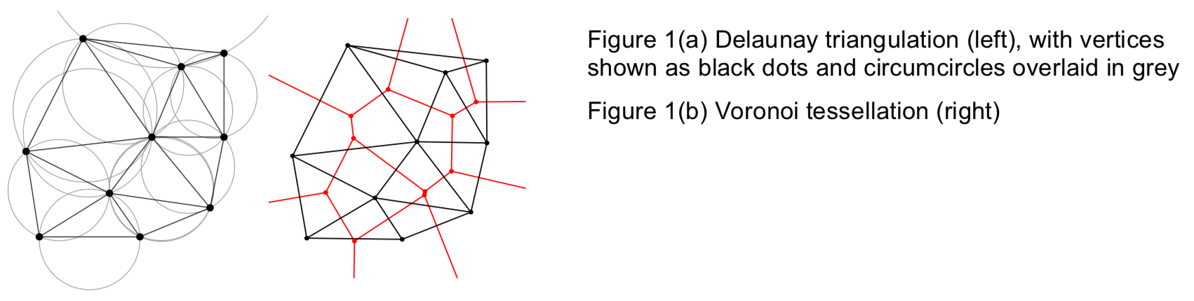
To triangulate, we use the Delaunay technique [DELAUNAY 1934; WIKIPEDIA] that is well known in computational geometry. The Delaunay technique does not necessarily give triangles of maximum area; however, it gives a set of well-shaped triangles where the minimum angle at every vertex is maximized: It does not produce slivers.
We represent the triangulation using two data structures. The first structure comprises a list of vertices; each vertex entry contains the vertex coordinates (“lat/long”) and the corresponding (scalar) elevation. The second structure comprises a list of triangles; each triangle is represented as a set of three vertex indices.
To interpolate elevation values within each triangle, we form a weighted average of elevations carried at its vertices. One method of doing so is to use distances to the vertices as weighting factors. Another method of doing so is to use barycentric interpolation: a coordinate 0 through 1 is assigned along each triangle edge; the interior point to be interpolated is described in those coordinates, which are taken to be the weighting factors. Both schemes work adequately well, but have the disadvantage that although the interpolated values are continuous across triangle edges (C0 continuity), the first derivatives are not; the interpolated values are not as smooth as we would like. We seek an interpolation scheme that provides continuity of not only the function but also its first derivative (C1 continuity). To achieve that, we use Voronoi tesselation.
Our convex hull is the envelope containing all of the vertices. Using the interior vertices, we have triangulated the space within the convex hull. Obviously, triangular regions are formed. We can partition the space to form a region surrounding each vertex such that all of the points in each region have that vertex as their nearest neighbour. This process of partitioning is called Voronoi tessellation [VORONOÏ 1908; WIKIPEDIA; MATHWORLD]; it forms Voronoi cells (which in the 2-D case are polygons). Voronoi tessellation forms a geometric structure that is the dual of triangulation: each vertex in the triangulation is associated with a region in the tessellation, and each triangle edge is associated with an edge in the tessellation. Computational geometers have devised several algorithms that perform Voronoi tessellation quite efficiently [AURENHAMMER 1991].
The answer to obtaining C1 continuity in our interpolated values is to use the areas of neighbouring Voronoi cells as our weighting factors. The scheme is called natural neighbor interpolation; Amidror [2002] has written an excellent summary of the scheme. Both distance-based interpolation and barycentric interpolation fail to provide C1 continuity; in addition, both are liable to have the interpolation result unduly affected by points outside their logical region of influence. Natural neighbour interpolation offers C1 continuity, and in addition, behaves well in both clustered and sparse regions of data points.
Our terrain-map example has 2-D coordinates (lat/long); a scalar quantity (elevation) is either available (at a measured vertex) or interpolated (at points where no measurement is available). The terrain map is a function of two real variables and returns a real; in the language of mathematics it is denoted f :R2 ↦ R. The colour calibration problem has 3-D coordinates; it maps a triplet to a triplet. The mapping is denoted f :R3 ↦ R3. Triangles in the 2-D example become tetrahedra in our colour problem; instead of triangulation, we must perform tetrahedralization. Area in the 2-D example becomes volume in our colour problem. The Delaunay and Voronoi concepts both generalize from 2-D to 3-D.
Extending our 2-D terrain map example to 3-D colour calibration, the two basic data structures mentioned earlier are expanded. In colour calibration, each entry in the vertex list comprises a pair of triples: device data, and measurements transformed to what we call signal data. Each tetrahedron is associated with four vertex indices. Other data structures are required to represent the Voronoi tessellation. We compute and store the volume of each Voronoi cell. When measurement data is to be interpolated at a point within a tetrahedron, the volumes of the Voronoi cells associated with each of the tetrahedron’s vertices, suitably normalized, are used as weighting factors in the interpolation.
Conclusion
We have described how to construct 3-D colour lookup tables (LUTs) that are suitable for use with hardware, firmware, and software systems that use tetrahedral interpolation to calibrate display devices to studio standards. Our technique uses the Delaunay and Voronoi concepts that are well known in computational geometry to implement natural neighbor interpolation. The technique achieves smoother and more accurate mappings than are possible with trilinear or tetrahedral interpolation techniques.
Acknowledgment
We thank Mark Schubin for his thoughtful and timely review of a draft of this article. We also thank our SpectraCal colleagues L.A. Heberlein, Derek Smith, and Joshua Quain.
References
- 1. AKIMA, HIROSHI (1970, Oct.), “A new method of interpolation and smooth curve fitting based on local procedures,” J. ACM 17 (4): 589–602.
- 2. AMIDROR, ISAAC (2002, Apr.), “Scattered data interpolation methods for electronic imaging systems: A survey,” in J. Electronic Imaging 11 (2): 157–176.
- 3. AURENHAMMER, FRANZ (1991), “Voronoi diagrams – A survey of a fundamental geometric data structure,” ACM Computing Surveys, 23 (3): 345–405.
- 4. CIE 159 (2002), A Colour Appearance Model for Colour Management Systems: CIECAM02.
- 5. DELAUNAY, BORIS N. (1934), “Sur la sphère vide. A la mémoire de Georges Voronoï,” in
- Bulletin de l’Académie des Sciences de l’URSS, Classe des Sciences Mathématiques et Naturelles, No 6: 793–800. (His surname is also spelled Deloné, or in Russian, Делонé.)
- 6. FAIRCHILD, MARK D. (2005), Color Appearance Models, Second edition (Wiley).
7. MATHWORLD, Voronoi Diagram <https://mathworld.wolfram.com/VoronoiDiagram.html>. - 8. POYNTON, CHARLES (2012), Digital Video and HD Algorithms and Interfaces, Second edition (Elsevier/Morgan Kaufmann).
- 9. POYNTON, CHARLES, and FUNT, BRIAN (2014, Feb.), “Perceptual uniformity in digital image representation and display,” in Color Research and Application 39 (1): 6–15.
- 10. VORONOÏ, GEORGY F. (1908), “Nouvelles applications des paramètres continus à la théorie des formes quadratiques,” in J. für die Reine und Angewandte Mathematik 133: 97–178.
- 11. WIKIPEDIA, Voronoi diagram <https://en.wikipedia.org/wiki/Voronoi_diagram>.
- 12. WIKIPEDIA, Delaunay triangulation <https://en.wikipedia.org/wiki/ Delaunay_triangulation>.